We’re learning how to perform multiple regression analysis using stata this session. Regression is a prominent statistical technique for predicting a single outcome variable (continuous variable) from a set of independent factors (continuous as well as binary variables). For example, you may use gender (binary), family income, age, parental education, and self-efficacy to predict pupils’ academic success (GPA on a scale of 1-4). (all continuous). The presence of numerous independent variables in a single model gives researchers the confidence to draw conclusions while accounting for other factors that may influence academic success. Correlation, ttest, and anova provide results based on a one-on-one relationship, as you may recall (or bivariate relationship). These bivariate analyses, on the other hand, are valuable for us since they provide a descriptive picture of the data.
Let’s take a look at the data we utilized in our ANOVA analysis previously. Let’s imagine we want to predict academic achievement based on a few other variables like gender, age, mother and father’s education, computer lab use, and parental participation. The command “regress” or “reg” for short is used for multiple regression. Your result variable comes after “reg,” followed by the remainder of your independent variables. This is how it appears: edumom edudad labuselast parentinvolvement, beta reg rank gender age edumom edudad labuselast parentinvolvement
Preparing Data for Regression Analysis
Outliers can affect regression analysis. Here’s how I’d handle the following variables. However, before we begin any analysis, we must first verify the distribution of the variables we’ll be using. You’ll need to check to see if any of your variables are skewed. Outliers can affect regression analysis. So, we have to prepare our data for multiple regression analysis using stata software.
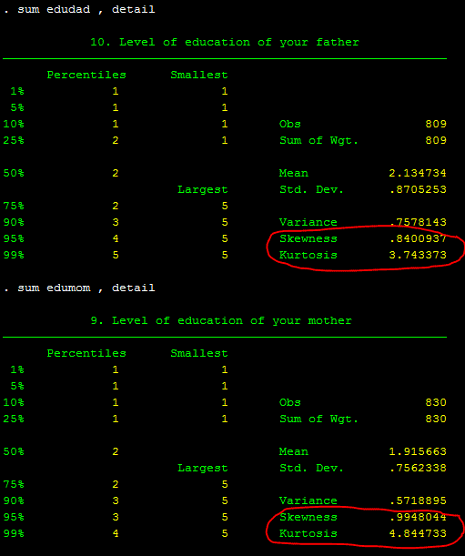
As you may be aware, the tab will provide percentages for each response, while the detail will display the skewness value. As you recall from the previous class on variable manipulation, a normally distributed variable should have a skewness of one or less (closer to zero is better) and a Kurtosis of less than three. Please see this website for more information on skewness and Kurtosis. Except for edumom and edudad, all of these factors appear to be in good shape. See below of the breakdown by each level of education when using tab command:

As you can see, just a few fathers (only ten) have completed high school, and the situation is even worse for mothers (only a few of them have completed high school (3.73 percent) and above high school education (.60 percent)). It appears to be skewed. You can also check for skewness by using sum, detail.

What options do we have?
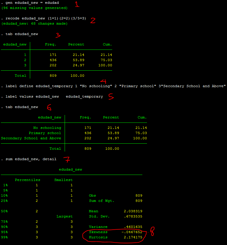
Recoding these two variables and then rechecking the skewness is the best method. Let’s start with recoding the edudad, and then you can work on recoding the edumom on your own. As you may be aware, it is recommended that you create a new variable and utilize it before recoding any variables. This way, you may maintain your previous variable in case you need to go back later. Below is a video of the entire process:

Those are the 8 steps I would do to recode one variable and to check the skewness of that variable. As you can see, the skewness is reduced to almost zero, and Kurtosis to lower than 3.
Multiple Regression Analysis
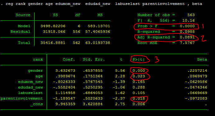
reg rank gender age edumom_new edudad_new labuselast parentinvolvement , beta
Interpretation of Multiple Regression Analysis
The whole regression model with all of these factors is statistically significant, as shown by the regression output above: F(6, 556)=10.16, p.001, Adjusted R-squared =.09. So, look at the likelihood (#1), then R-squared or Adjusted R-squared (#2), and, if the #1 is significant, individual p values of each predictor (#3). The adjusted R-squared of.09 indicates that the independent variables in the model explain for 9% of the variance in the outcome variable. When you have a lot of independent variables in your model, adjusted R2 is preferable because it accounts for the amount of variables in the model.
R2 tends to increase as you add more variables to the model, therefore using modified R2 to ensure that the variables you include in the model are useful (i.e., not just junk) is a good idea. R2 or adjusted R2 also shows effect size, with bigger R2 values indicating larger effect sizes and thus more desirable results. According to Cohen (1988), the average effect size in social science domains is medium.
Gender (beta=.23, p.001), age (beta=.10, p.05), and parental engagement (beta= -.10, p.05) are all significant predictors, according to the regression output. It’s worth noting that if the Prob>F isn’t significant, you don’t have to provide the important predictors.
Output table
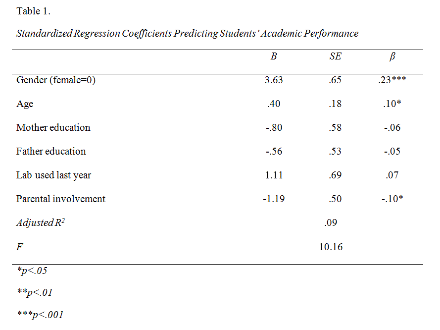
This is an example of how “multiple regression analysis using stata” table and the write up look like based on the above regression output:

“Table 1 shows that the overall model was significant, F(6, 556)=10.16, p<.001, Adjusted R2=.09. The model explains 9% of variance accounted for by the predictor variables. Factors that predict academic performance include gender (β=.23, p<.001), age (β=.10, p<.05), and parental involvement (β= -.10, p<.05). Specifically, the results suggest that being female, being younger, and having parents who are more involved are significantly associated with better academic performance.”